High Throughput Calculation (HTC): Pattern Compositions
Purpose: Learn to run high throughput calculation by setting pattern composition range and steps.
Module: PanPhaseDiagram
Thermodynamic Database: AlMgZn.tdb
Calculation Procedures:
-
Load AlMgZn.tdb following the procedure in Pandat User's Guide: Load Database, and select all three components;
-
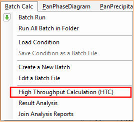
Choose the HTC function from the menu "Batch Calc → High Throughput Calculation (HTC)" (as shown in ).
-
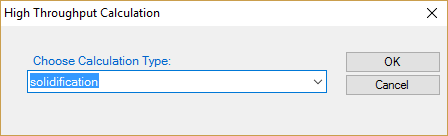
Choose the calculation type from the drop-down list of HTC pop-up window and select “Solidification”.
-
Define the compositional space for HTC simulation;
-
Save the current workspace after all calculations are finished. It is suggested that user saves the current workspace immediately after the HTC calculation. This allows all the calculated results saved in the workspace for future use.
-
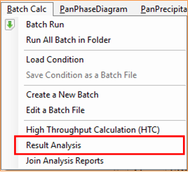
Choose “Result Analysis” from the “Batch Calc” menu. User can use this commend to analyze the calculated results for a group of alloys and pick a certain property from each calculation for comparison.
-
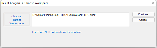
Open the workspace saved previously for “Result Analysis”. User can perform several HTC calculations and save all the workspaces. User can then analyze the results of the selected HTC calculation by opening the corresponding workspace as shown in Figure 5.
-
Define the criteria of the properties as filters for result analysis
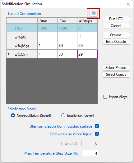
After choosing the calculation type, a window pops out as shown in Figure 3. In this setting, the compositions of both Mg and Zn vary from 1 to 30 wt.% in a double composition loops. The “Steps” is set to 29, which means the composition increases by 1 wt% at each step. The total number of calculations is 30x30=900 in this setting. The composition of Al is set as balance by typing “-1” for steps or right-click the row of Al. No “Start” or “End” values are required for the balance component, which is Al in this case. After setting the composition pattern, user can also export these HTC alloy composition to a file by clicking the small icon marked with red square in Figure 3 After setup the compositional space for HTC and choose the proper solidification model, user can click “Run HTC” button to perform HTC simulations, which is 900 calculations in this case.
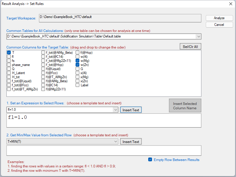
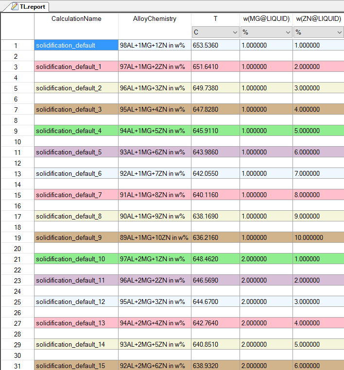
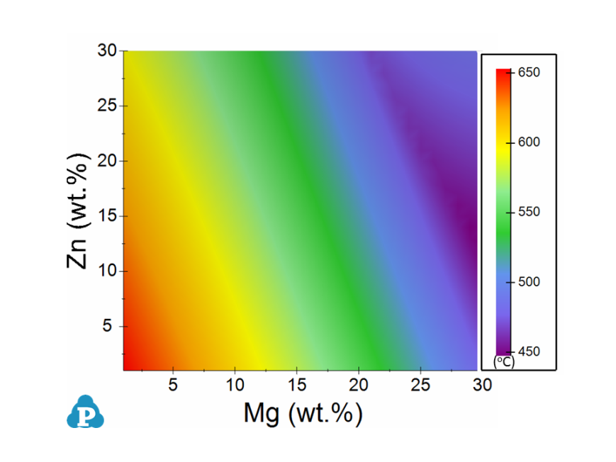
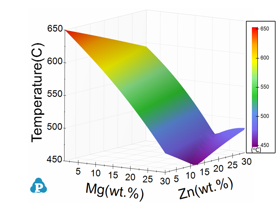
In Figure 6, the “Target Workspace” shows the workspace selected by the user for results analysis. It should point out that there can be more than one table in each calculation, the “Common Tables for All Calculations” allows user to choose the table for analysis. In the “Common Columns for the Target Table” window, names for all the output properties available in the selected table are listed. User can choose the properties to be listed in the “Analysis Report”. As shown in Figure 6, temperature and the alloy composition will be listed in the “Analysis Report” in this case. Since the purpose of HTC is to compare a special target property for the several hundred/thousands of calculations, the “Set an Expression to Select Rows” at the bottom of the window allows user define the criteria. In Figure Figure 6, this criterion is fL=1, i.e. the fraction of liquid is 1. With this filter, only the row satisfies this criterion will be listed in the “Analysis Report”. It should point out that several criteria can be set in the “Set an Expression to Select Rows”. Click “Analyze” to create the “Analysis Report” as shown in Figure 7. In this table, each row lists the liquidus temperature for the corresponding alloy composition. The liquidus temperatures for 900 alloys are listed in the same report which allows a quick comparison of liquidus temperature for different alloy composition. User can also plot 3D colormap and surface diagrams using the data in this report as shown in Figure 8.